
Did the New Nature Study Correct Away Evolution in Ancient Europe?
Why ancestry, geography, and polygenic scores do not move through ancient Europe as one simple line.

TL;DR: Akbari et al. model ancient West Eurasia with a single ancestry-corrected time trend. But the data do not look like one trend. WHG, EEF, and Steppe ancestry follow different temporal and geographic trajectories, and the PGS slopes differ by ancestry background. This means the method can miss not only between-group historical change, but also ancestry-specific within-lineage change. Correcting for ancestry is useful, but in ancient DNA it can also correct away part of the evolutionary history one is trying to study.
Ancient DNA has made one old temptation harder to resist. Once we can line up skeletons by date, plot their polygenic scores, and watch some traits move across thousands of years, it is natural to talk about a single trend through time.
That is also how the recent Akbari et al. selection scan is framed statistically. Their core model estimates one time coefficient for each trait after correcting for genome-wide relatedness. That is a clear and useful estimand, but it raises a question: what if ancient West Eurasia does not have one temporal trend?
Europe was not a single biological conveyor belt. The people sampled at 10,000 BP, 5,000 BP, and 2,000 BP were not just earlier and later versions of the same population. They carried different proportions of ancestry related to western hunter-gatherers, early European farmers, Steppe pastoralists, and later historical mixtures. If those ancestry backgrounds also had different trajectories, then a single time coefficient will compress too much history into one number.
That is what I wanted to test here. The question is not only whether polygenic scores changed through time. The sharper question is whether the single-trend assumption is adequate: did PGS trajectories move in the same way across ancestry backgrounds, or did different ancestries carry different slopes through time?
Very Short Methods Note
I used ancient West Eurasian individuals from AADR v66, restricted to samples from the last 18,000 years with K7 ADMIXTURE components available. The analysis sample contains 11,102 ancient individuals. Time is coded so that higher values mean more recent samples. The three ancestry components highlighted here are WHG (Western Hunter Gatherers), EEF (Anatolian/Early European Farmers), and Steppe_Yamn_CW (Steppe/Yamnaya/Corded Ware). I modelled each component as a function of time, latitude, longitude, and their interactions. I then tested whether the time slope for polygenic scores differs by ancestry background using models of the form:
PGS ~ time + ancestry component + time x ancestry component + latitude + longitude + coverage
The polygenic scores are standardized. EA is educational attainment, Height is height, and DD is delay discounting. DD is exploratory because the underlying score is much sparser than EA or Height.
The Ancestry Background Changes Sharply Through Time
The ancestry composition of the sample is strongly time-structured. WHG is high in the oldest bin, EEF rises after the spread of farming, and Steppe ancestry rises sharply after 5,000 BP.
Table 1 gives the basic time-window summary. The values are mean ADMIXTURE component proportions, so they should be read as broad ancestry signals rather than literal population labels.
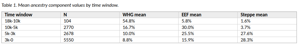
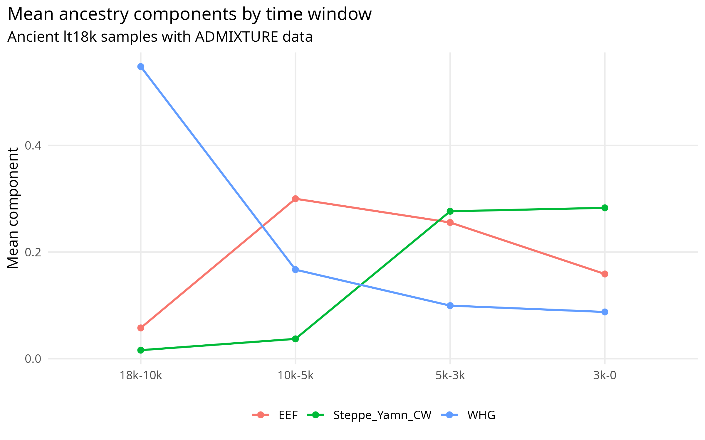
The same pattern is easier to see visually. Figure 1 shows the turnover directly: the oldest samples are WHG-heavy, the middle Holocene samples are much more farmer-related, and the later samples carry much more Steppe-related ancestry.
Figure 1. Mean WHG, EEF, and Steppe ancestry components by time window.
The Steppe Increase Is Not Just a Date Effect
The Steppe component increases toward the present even after controlling for latitude and longitude. The adjusted slope is positive and large. EEF and WHG move in the opposite direction.
The spatial interactions are important. Steppe ancestry increases more strongly at higher latitude and toward the west. EEF and WHG decline toward the present, but their decline is structured more by longitude than by latitude.
Table 2 reports the core regression results. The first numeric column is the time slope after latitude and longitude are included. The interaction columns ask whether that time slope changes at different latitudes or longitudes.
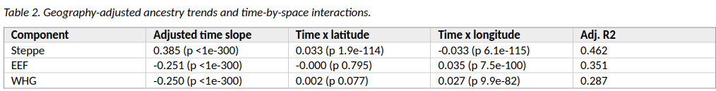
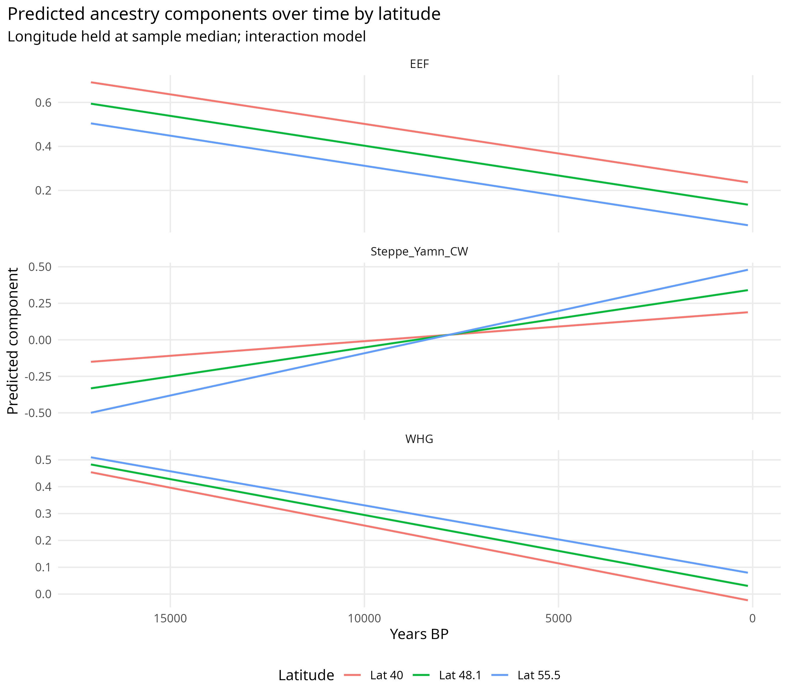
Figure 2 then turns those interactions into predicted ancestry trajectories. It is useful because it shows that the Steppe rise is not evenly distributed across space.
Figure 2. Predicted ancestry components through time at different latitudes.
The ancestry turnover alone already makes the single-trend assumption look fragile. But the more important question is whether this matters for the polygenic scores themselves.
Below I test that directly: first by asking whether ancestry components change the PGS slopes through time, and then by decomposing the signal into within-group and between-group components. This is where the Akbari-style correction becomes most interesting.
