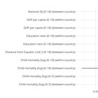
Correction, August 29, 2025: A previous version was accidentally sent. It misinterpreted the education ratio. The ratio is male to female, so a negative coefficient means higher female to male education is associated with higher fertility. This version corrects the text and figures.
In my previous
articles I used Mundlak within-between models, which compare cohorts within the same country to their long-run average childhood conditions. Those models showed robust effects: higher life expectancy and GDP in early life (0-18) predicted lower fertility, while adulthood shocks pointed the other way (higher mortality → higher fertility via replacement). For education, the correct interpretation is that higher female-to-male education (that is, a lower male-to-female ratio) was associated with higher fertility in the 18-45 window.
But what if we think of this as a time series problem? Cohort fertility doesn’t jump randomly from one level to the next, it is highly persistent. To capture that, I re-estimated the same windows with a dynamic panel model (system GMM), treating fertility as a process where each cohort’s completed fertility depends heavily on the one before it.
Why dynamic panels?
Persistence: fertility is sticky; ignoring that risks over-attributing changes to covariates.
Lag structure: dynamic GMM includes lagged fertility (CCF_{t-1}) as a regressor, instrumented with deeper lags to avoid bias.
Different question: instead of “do cohorts exposed to worse/better conditions differ in fertility?” (Mundlak), the time-series angle asks: conditional on the last cohort’s fertility, do these shocks still matter?
The diagram below illustrates the differences between the two methods.
Results at a glance
Interpretation note: the education ratio is male-to-female. Negative coefficients mean that higher female-to-male education is associated with higher fertility.
Childhood windows
0-14
Coef ≈ –0.43* (p = 0.040) in life-only spec
Coef ≈ –0.57 (p = 0.055) in child-mort-only spec
Coef ≈ –0.75 (p = 0.090) in GDP-only spec
➝ Negative, sometimes significant at ~5–10% level → implies higher female-to-male education is linked to higher fertility.
0-18
Coef ≈ –0.52* (p = 0.012) in life-only spec
Coef ≈ –0.67 (p = 0.063) in child-mort-only spec
Coef ≈ –0.84* (p = 0.043) in GDP-only spec
➝ Consistently negative, significant in multiple specs → higher female-to-male education associated with higher fertility.
0-25
Coef ≈ –0.75* (p = 0.011) in life-only spec
Coef ≈ –1.04* (p = 0.035) in child-mort-only spec
Coef ≈ –0.95 (p = 0.082) in GDP-only spec
➝ Strongly negative, often statistically significant → same interpretation.
Adult window (18-45)
18-45
Coef ≈ +0.35 (p = 0.320) in GDP-only spec
Coef ≈ +0.31 (p = 0.172) in life-only spec
Coef ≈ –0.87 (p = 0.206) in child-mort-only spec
➝ Mixed signs, none significant.
Across all windows (0-14, 0-18, 0-25, 18-45)
Lagged fertility dominates. The coefficient on CCF_{t-1} is ≈ 1.0 across the board, highly significant. Cohort fertility is almost entirely explained by inertia.
GDP, life expectancy, and child mortality mostly vanish. Once persistence is controlled for, their coefficients shrink toward zero and lose significance. For example, the Mundlak model gave strong negative early-life effects of life expectancy and child mortality, but the dynamic model yields estimates near zero (ns).
Education ratio is the one exception. In childhood windows it often shows a large, negative coefficient (–0.5 to –1.0), implying that higher female-to-male education is associated with higher fertility, though these estimates are not perfectly stable and the p values are close to 0.05 (all >0.01).
Adult exposures (18-45) flatten out. GDP and life expectancy flip slightly positive, child mortality loses significance.
Overall pattern
Childhood exposure windows (0-14 / 0-18 / 0-25): education ratio coefficients are consistently negative. Because the ratio is male-to-female, this implies higher female-to-male education is associated with higher completed fertility, with effect sizes around –0.5 to –1.0 and several results significant at p < 0.05.
Adult window (18-45): effects are inconsistent and not significant.
Conclusion
The apparent tension between the Mundlak within-between results and the dynamic panel estimates isn’t a contradiction, it is a difference in what trend each model is testing. Mundlak decomposes country-cohort outcomes into deviations from each country’s long-run average, so it asks a cross-cohort question: do cohorts that grew up under worse (or better) childhood conditions end up with different fertility levels relative to their country’s norm? By contrast, the dynamic panel (system GMM) treats fertility as a persistent time series and conditions on the prior cohort’s fertility. It asks a short-run question: given where the last cohort ended up, do shocks in childhood or adulthood still move fertility further up or down? Because these estimands target different trends (long-run level differences vs. incremental changes around an autoregressive path), different answers are expected.
Once we account for persistence, inertia dominates: the lagged term is ~1 and highly significant across windows, and coefficients on GDP, life expectancy, and child mortality largely shrink toward zero. That doesn’t invalidate the Mundlak findings, it says those variables help explain long-run level differences across cohorts within countries, but contribute little to additional movement once the path is set. The partial exception is education: in childhood windows the negative coefficients on the male-to-female ratio imply that greater female relative education is linked to higher fertility, while adulthood exposures are mixed and not significant. Notably, this mirrors the opposite emphasis in my Mundlak runs, where education’s strongest signal appeared in the 18-45 window, and where lower relative female education (higher male to female education ratio) had a positive effect on fertility.
Taken together, the dynamic panel results contradict the uncorrelated.xyz findings and most coefficients are imprecise, which suggests this methodology is not ideal for capturing slow-moving, long-term trends in cohort fertility. The lagged dependent variable absorbs most of the variation, so signals from childhood exposures and education balance are muted. Mundlak within-between models speak more directly to level differences across cohorts, which is closer to the long-run question. In light also of the literature showing a negative effect of female education on female fertility across individuals (within countries), the effect from the Mundlak within-between models are more credible.
My read is that dynamic GMM is useful for short-run adjustments, not for identifying secular trends.
Specification note. The dynamic panel models were estimated with system GMM (Arellano–Bover/Blundell–Bond) using plm::pgmm
. I specified lagged CCF(t–1) as a regressor and used lag 2 of CCF as the GMM instrument (collapsing the instrument matrix to keep it parsimonious). Covariates (GDP, life expectancy, child mortality, education ratio) were treated as standard instruments. Robust standard errors were reported. Hansen test p-values were comfortably above conventional thresholds, suggesting the instrument set is not overfitting, and AR(2) tests did not reject the null of no second-order serial correlation.
Have you enjoyed this post? Please subscribe or refer a friend!