
When Correcting for Ancestry Corrects Away Evolution

Ancient DNA selection scans often follow a simple rule: first correct for ancestry, then see what remains. That sounds sensible. Nobody wants to confuse population structure with selection.
But in ancient DNA, ancestry is not a nuisance variable like a genotyping batch. It is part of the historical process. The populations of West Eurasia did not sit still while time passed over them. Hunter-gatherer ancestry, early farmer ancestry, Steppe ancestry, and later historical mixtures all entered the record at different times and in different places.
That creates a problem for any model that tries to reduce ancient West Eurasia to one corrected time trend.
Akbari et al. ask whether polygenic scores changed through time after controlling for genome-wide relatedness. That is a useful question, but it is not the same as asking whether populations evolved through time. If sampling date is correlated with genetic structure, then a GRM correction can absorb both confounding and genuine historical signal. Worse, if the corrected coefficient is interpreted as individual-level selection, the estimate depends on an exogeneity assumption that may be violated.
TL;DR: Akbari et al.’s method is not useless. It answers a narrow residual question: is there a time trend after genome-wide structure is absorbed? But the broader evolutionary question is different. Much of the signal is between ancestry-like groups, and even within groups the slopes may not be common across ancestry backgrounds. Correcting for ancestry can therefore correct away part of the evolutionary history one is trying to study.
What Akbari et al. did
The core model can be written roughly as:
PGS_i = alpha + gamma * time_i + genetic_relatedness_random_effect_i + error_i
The genetic relatedness term is based on a genome-wide relatedness matrix, or GRM. This matrix summarizes how genetically similar every individual is to every other individual; mathematically, it captures the same broad structure that appears in genetic principal components, but the model uses the GRM as a covariance matrix rather than adding a few PCs as ordinary covariates. Its purpose is to account for the fact that ancient individuals are not independent draws from one homogeneous population. Related individuals and genetically similar groups should not be allowed to manufacture a fake time trend.
That is a reasonable concern. But the resulting `gamma` is not the total temporal change in the trait. It is the residual time trend after genome-wide structure has been absorbed.
Why This Is Not the Same as Total Evolution
Suppose a trait-related PGS rises through time because one ancestry background partly replaces another. Is that confounding, or is that evolution?
The answer depends on the question. If the question is narrowly, “Did the score change within a fixed genetic background?”, then ancestry turnover is something to remove. But if the question is, “Did populations genetically change through time?”, then ancestry turnover is one mechanism by which the change occurred.
That is the first limitation of the Akbari-style correction. It can remove a historically meaningful group component by treating it as structure.
The Stronger Statistical Issue
There is a second issue. Random-effects-style identification depends on the random effect not being correlated with the explanatory variable. Here the explanatory variable is time. In ancient DNA, time is obviously correlated with genetic structure: older samples and younger samples are not drawn from the same ancestry distribution.
The point is not merely philosophical. If the genetic random effect is correlated with sampling date, then the corrected time coefficient may not cleanly estimate the individual-level selection parameter. If there is correlation of this type, then the parameter estimate obtained is biased and inconsistent.
Prof. Gregory Connor pointed out this problem in the Akbari et al. methodology in an earlier tweet. [


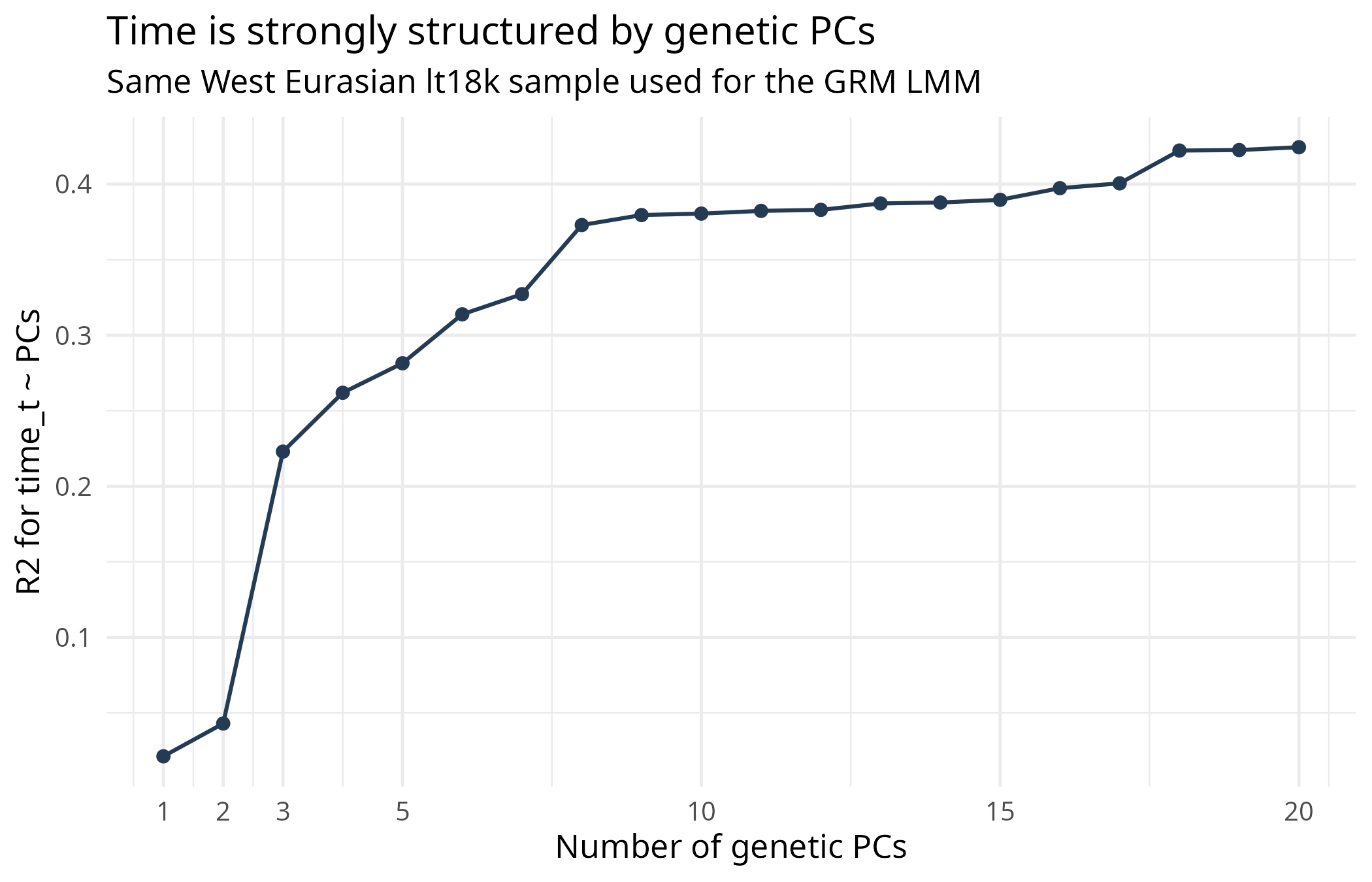
The data show the dependence directly. Genetic PCs predict sampling time; the first ten PCs explain about 38 percent of the time variable.
Figure 1 shows the same diagnostic visually. This is the background fact behind the whole problem: date is genetically structured.
If genetic structure predicts date, then a structure-corrected time coefficient is not automatically a clean individual-level selection estimate.
Figure 1. Genetic PCs predict sampling time.
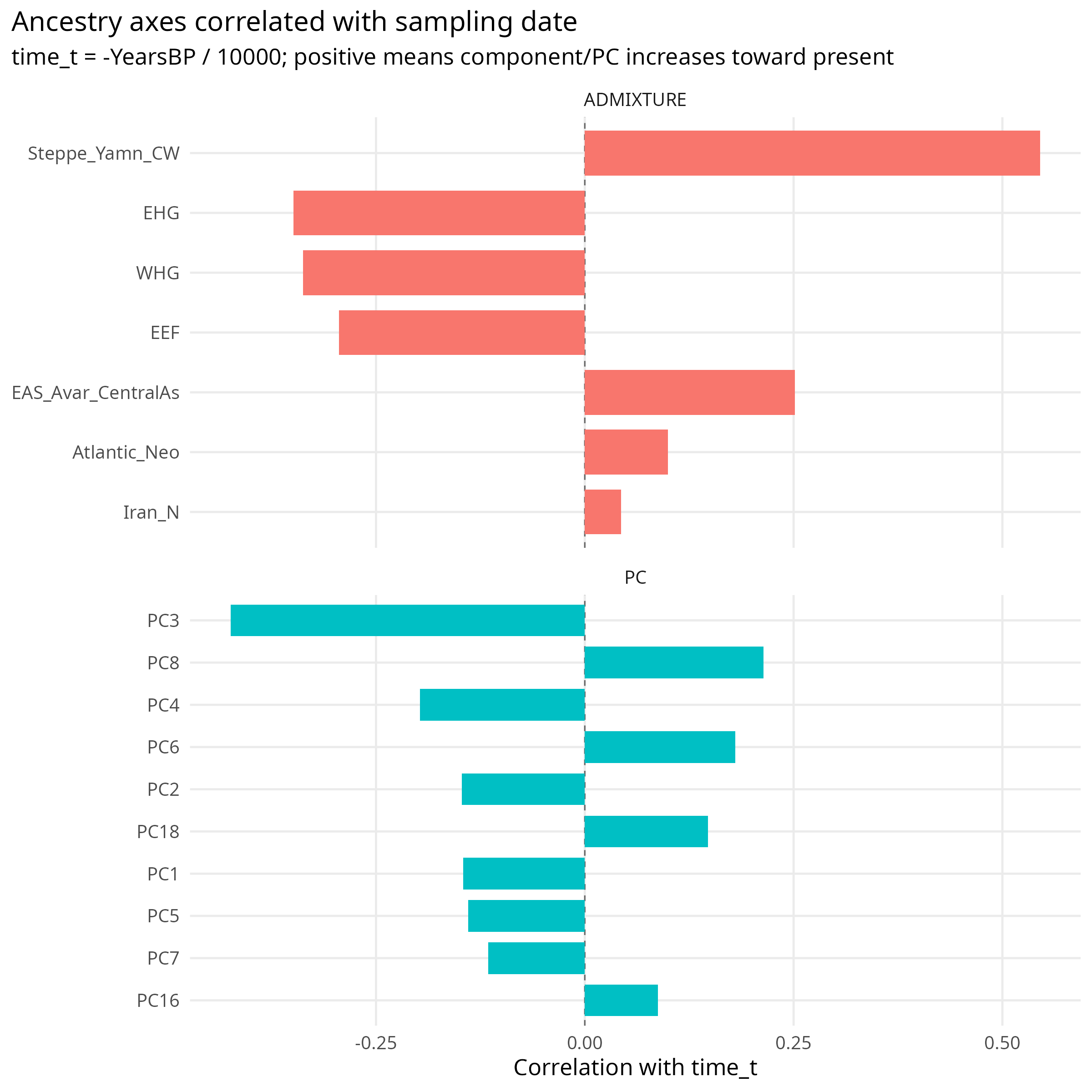
ADMIXTURE components tell the same story. Steppe ancestry rises toward the present, while WHG and EEF are older-enriched. This is not a minor nuisance; it is the central structure of ancient West Eurasian history.
Figure 2. Correlations between sampling time, genetic PCs, and ADMIXTURE components. Time is not independent of genetic structure.
Fixed Effects as a Check
A possible solution is to estimate fixed effects. Fixed effects ask a narrower question:
Within the same group, do later samples have different PGS than earlier samples?
They do not use between-group differences to estimate the time slope. That is the tradeoff. Fixed effects cannot estimate the part of evolution that happened through group turnover, but they can estimate within-group temporal change.
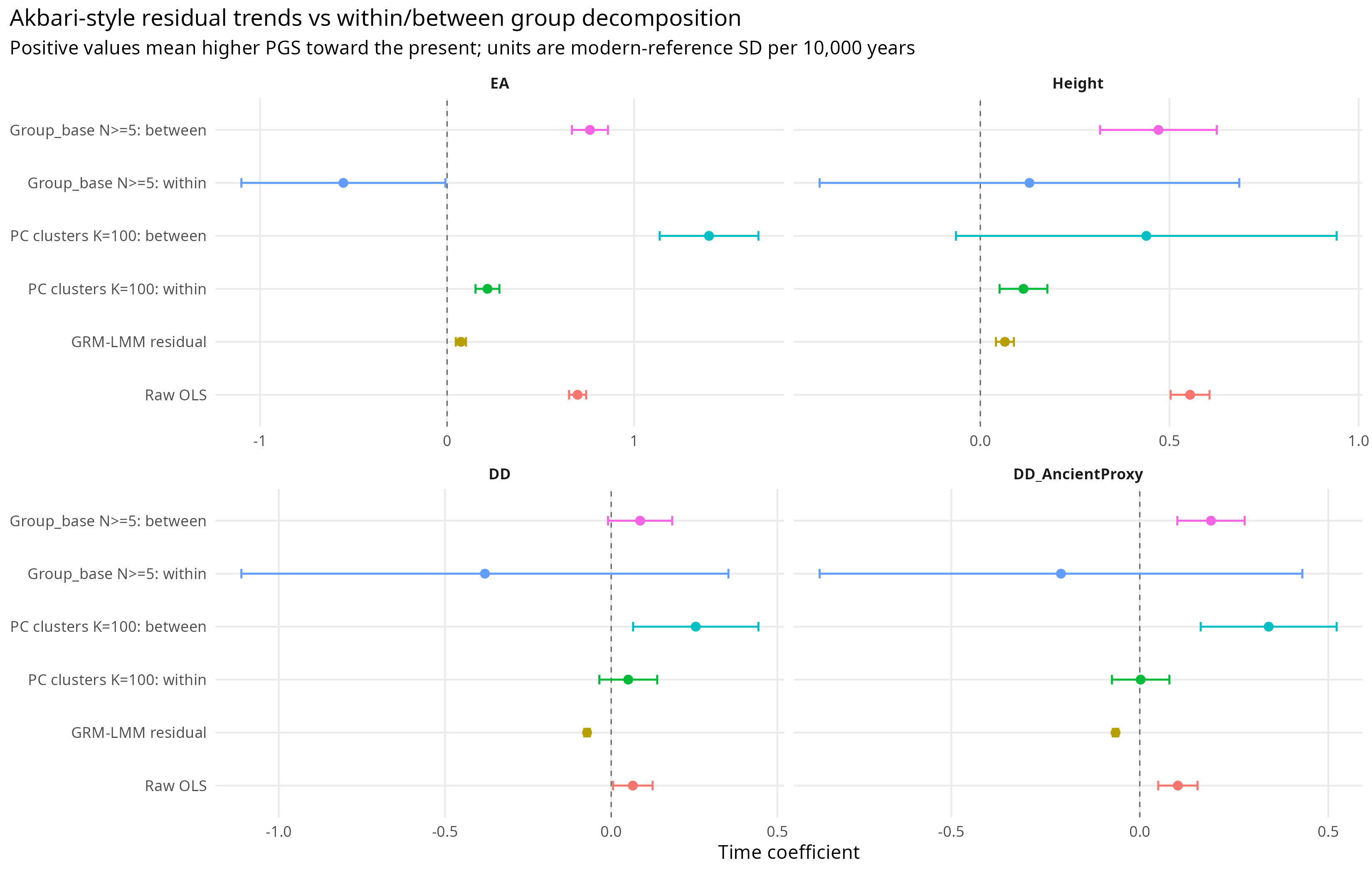
Using ancestry-like PC100 clusters, the fixed-effects estimates remain positive for EA and Height. They are smaller than pooled OLS, but larger than or comparable to the GRM-LMM estimates.
Table 2. Pooled OLS, GRM-LMM, fixed effects, and Mundlak between-group estimates.

For EA, pooled OLS gives a gamma of 0.698. The GRM-LMM estimate is 0.074. The PC100 fixed-effects estimate is 0.216. That means the within-cluster signal is still present, but the GRM correction estimates a much narrower residual trend.
For Height, pooled OLS gives 0.554, GRM-LMM gives 0.065, and fixed effects give 0.114. The same pattern appears, though less dramatically.
How Large Are the Group Effects?
The Mundlak decomposition makes the group component explicit:
PGS_ig = alpha + beta_within * (time_ig - mean_time_g) + beta_between * mean_time_g + error_ig
The within coefficient asks whether samples change through time inside ancestry-like clusters. The between coefficient asks whether clusters with different average dates also differ in PGS.
For EA, the within-cluster gamma is 0.216. The between-cluster gamma is 1.401. The between-group temporal gradient is therefore about 6.5 times larger than the within-group gradient.
For Height, the within-cluster gamma is 0.114 and the between-cluster gamma is 0.439, about 3.8 times larger.
Table 3. Size of the between-group temporal component using PC100 ancestry-like clusters.
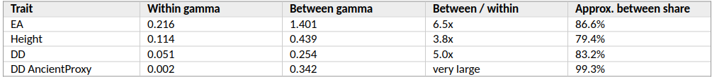
Figure 3 summarizes the same point graphically. The answer changes depending on whether the model estimates the raw trend, the residual GRM-corrected trend, or the within/between decomposition.
Figure 3. GRM-LMM and Mundlak-style decomposition of temporal PGS change.
What This Means
Akbari et al.’s method is not useless. It is useful for one narrow question: does a residual average time trend remain after genome-wide structure is absorbed?
But it should not be sold as the full story of evolutionary change. The discarded group component is not automatically confounding. It may be the evolutionary signal.
The stronger problem is that a single corrected time slope may also miss ancestry-specific within-lineage change. If different ancestry backgrounds have different temporal slopes, then a model with one `gamma` compresses multiple trajectories into a single average. That can make real lineage-specific change look smaller than it is.
So the limitation is twofold:
1. The GRM correction can wash away between-group historical change.
2. The single-slope design can miss within-group or lineage-specific change when slopes differ by ancestry. Estimating a single-slope design is not even statistically consistent if the reality is that there are multiple-slope trends.
In ancient DNA, ancestry is not just something to control for. It is one of the ways evolution entered the data.
References
Akbari, A., Perry, A., Barton, A. R. et al. Ancient DNA reveals pervasive directional selection across West Eurasia. Nature (2026). https://doi.org/10.1038/s41586-026-10358-1
Allen Ancient DNA Resource, AADR v66.2, Reich Lab.