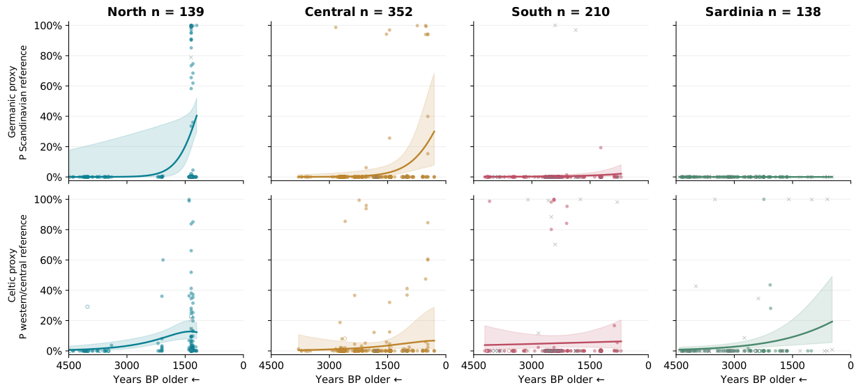
Adjusted probabilities through time in ancient Italy
Revised 6 November 2026. Trends refitted after source-identity reconciliation. See the prehistoric phase tests and source-alias audit.
How to read these values — Probabilities measure model support for four ancient reference classes. They are not ancestry percentages. The Italian comparator pools central Italian Etruscan, Picene and Latial Iron Age or Republican people. The geographical reference labels identify the genetic distributions used for these comparisons.
Figures 7–8 compare North, Central, South and Sardinia after adjusting for usable-marker count and observed-versus-imputed data. The regression uses all four reference probabilities together. South includes Sicily; Sardinia is separate. A South-mainland sensitivity excludes Sicily while retaining the Sardinian panel.
After five additional source-alias joins, the full model contains 982 dated people (North 186; Central 365; South 272; Sardinia 159). The 4,500 BP model contains 839 (North 139; Central 352; South 210; Sardinia 138). Eighteen undated people remain in the cohort audit. Source labels recover the region of 23 people previously left unspecified by the coastal-coordinate mapping.
Older samples are on the left and younger samples on the right: Years BP decreases from left to right. Dots retain individual variation after adjustment through fitted relative odds. The line is the model's adjusted mean; shaded bands are conditional 95% intervals clustered by site. Filled circles: imputed >0.1×; hollow circles: other imputed; grey crosses: observed-only. Search filters the dots; the fitted model and Table 6 retain their full cohorts.
Figure 8. Adjusted reference probability by Years BP
Table 6. Chronological association and sensitivity checks
| Model | Area | N in area | Sites in area | Change, pp / 1,000 BP | 95% CI | p | Holm p |
|---|
Positive estimates mean higher probability in older genomes. Fractional-model rows give the average derivative at observed ages and controls, rather than a constant change over every 1,000-year interval. Linear probability sensitivities use a different mean specification. Holm correction covers the sixteen outcome-by-area tests within each primary window. Confidence intervals condition on the upstream classifier. Table 6 includes a linear coverage check on all 617 qualifying people; the attempted joint fractional sensitivity did not yield a stable information matrix.
How the adjustment works, source checks and limitations
The joint fractional multinomial logit uses the four original P values as fractional responses, preserving zero and one values without pseudo-counts. Each area has its own intercept and age slope. The principal controls are log usable-marker count and imputation status, standardised to their pooled means within each fitted cohort. The PCs are not covariates: they generate the response probabilities. Coverage is used only for a separate robustness subset. Curves stop at each area's observed date limits; they can span unsampled intervals.
For an individual, adjusted probability q is proportional to the original p multiplied by exp(delta), where delta is the change in the fitted class index after standardising the controls. Normalising the four q values makes them sum to one and retains exact zero probabilities. The scatter and regression line serve different purposes: individual variation and the fitted conditional mean.
Spatial/site-clustered sandwich intervals allow within-cemetery dependence and use a t reference with G−1 degrees of freedom. They do not propagate uncertainty in the frozen PCA classifier or archaeological dates. Mean dates and documented contextual midpoints are used. Site/study sampling changes through time, so adjustment cannot identify an Italian population's migration rate. The northern historical association is concentrated at Collegno; omitting it and adding publication effects substantially weakens that association.
The secondary linear probability model adds publication/source-category fixed effects. Thirty-four people have an unresolved publication label after source checks and remain under explicit accession/data-source categories; none is excluded for that reason. Four lack documented genome-wide depth and remain in primary models. Original source documentation establishes that the two PRJEB58428 six-column coverage values are target-panel depths; their genome-wide depths (0.0712× and 0.3399×) replace them only in the new regression coverage inventory.
The two recent South probabilities above 0.5 for the Scandinavian reference are I17881.AG (Himera, 0.001640×) and I3686.AG (Pompeii, 0.001739×), both sparse observed-only genomes. Table 6 includes sensitivities omitting those two observations, alongside the all-eligible primary fits. The source audit lists the five highest probabilities for every outcome and area.
The attempted quadratic-time joint models did not satisfy the numerical convergence checks, and the high-coverage joint model had an ill-conditioned information matrix. These are documented technical limits rather than evidence that a biological effect is absent. All eligible people remain in the principal models, and the high-coverage linear sensitivity retains all 617 qualifying people and all four outcomes. No penalised final estimator or outcome deletion is used. A small temporary penalty is used only to initialise finite coefficients and is removed before final fitting and inference. The inherited classifier has incomplete target-marker calibration for the new Italian class.
Method: Mullahy, Multivariate Fractional Regression Estimation of Econometric Share Models. Files: Table 6 CSV · individual adjusted values · source corrections · Figure 7 SVG · Figure 8 SVG